Fast polymer sampling, Part I: Markov chains and hash maps
This series of posts discusses the computational problem of sampling a mathematical model of linear polymers (as opposed to, e.g. branched polymers) known as the self-avoiding walk. In this post, I’ll introduce the problem, discuss some of the challenges it presents, introduce a general MCMC algorithm (known as the pivot algorithm) to tackle it, and show a simple implementation of this algorithm (in C++) that uses a hash table for collision detection.
In the next post, I’ll discuss a more sophisticated implementation of the pivot algorithm based on a tree-like data structure similar to the R-tree. In the final post, I’ll show how to squeeze out a little extra performance from this algorithm using a SIMD implementation of my own.
The model and problem
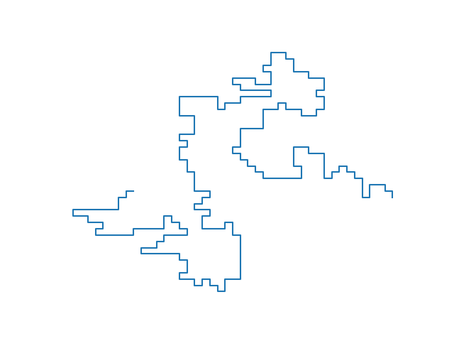
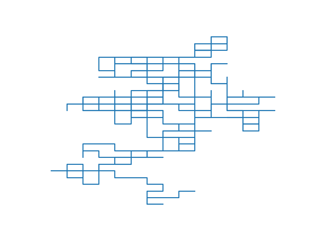
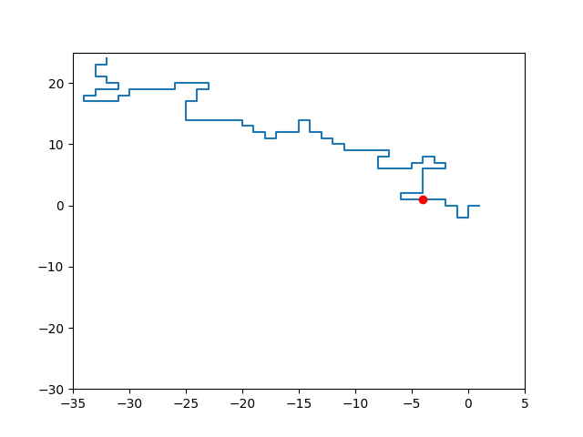
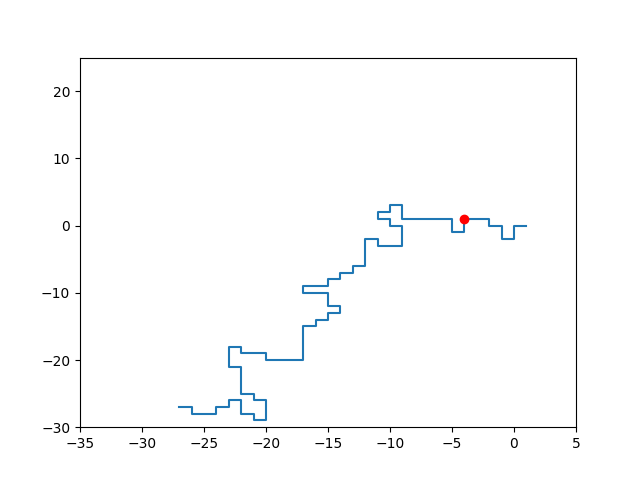
A (linear) polymer is a molecule formed by linking up a large number of smaller molecules, known as monomers. The self-avoiding walk (SAW) models this as a finite sequence of non-repeating adjacent sites on a lattice (I’ll stick to square/cubic/hypercubic lattices in this post), which we can visualize as being linked up by lattice edges (below left). In other words, a sample self-avoiding walk is similar to a (finite) sample of the simple random walk (SRW, below right) but the walk isn’t allowed to overlap itself (just as two monomers can’t occupy the same position in space). It’s really the simplest conceivable mathematical model for the physical phenomenon under question.
This series of posts discusses how to efficiently sample very large SAWs from the uniform distribution.
|
|
Disclaimer. My aim is to discuss the computational aspects of this sampling problem, specifically how to optimize for performance. I won’t go into the rigorous mathematics (analysis and proofs), physics (renormalisation arguments), or statistics (Markov chain mixing and autocorrelation) of this topic.
Statistical physics background
This section tries to provide some additional motivation for the problem of sampling from the uniform distribution over SAWs. If you’re already satisfied with the problem statement, feel free to skip it.
Statistical physicists like to study the properties of aggregate matter at equilibrium, which they do via probability theory. The idea of equilibrium can be summarized as follows:
-
A material has a set of states it might be found in when observed at a given moment.
-
As time passes, the material’s state evolves, tracking a trajectory through its state space.
-
Under appropriate conditions, the material will reach equilibrium, which is described by a time-independent probability distribution over possible states.
Equilibrium. Going back to polymers, which we imagine immersed into a fluid, suppose you’re able to force a given polymer into some particular state, such as a tightly curled up ball. Through random bombardment of the polymer by the molecules of its containing fluid, it will gradually move around and likely spread back out into a sort of random shape. At equilibrium, the SAW model assumes that any given (allowed) configuration of monomers is allowed and equally likely. In other words, the distribution under consideration is the uniform distribution over the (finitely many) SAWs of a given fixed size.
Scaling. The other key idea is that of studying aggregate matter, i.e. the focus on materials at “macroscopic” scales. In the case of SAW, this translates into studying the asymptotic properties of a uniformly sampled SAW of size \(n\) as \(n \to \infty\). To be more concrete, in this (and the following) post I’ll show how to sample a large number of SAWs of increasing size to determine a power law for the expected squared distance between a SAW’s origin and its endpoint.
Further reading.
-
A nice high-level overview of this model can be found in the following article:
Slade, G. Self-avoiding Walks. -
For the authoritative text on the subject:
Madras and Slade. The Self-Avoiding Walk.
The difficulty
So fixing a size \(n\), how do we sample a uniformly random SAW from the set of all SAWs of this size?
The remainder of this section discusses some ideas that don’t work. Feel free to skip to the next section if you want to see what does work.
Enumeration
The most straightforward way to sample from any finite set is to use an enumeration of every element in the set. However, it turns out the number of SAWs grows exponentially in \(n\) (indeed, all walks with strictly increasing coordinates are self-avoiding, and there are \(d^n\) such walks of length \(n\) in \(d\) dimensions). This will make exhaustive enumeration prohibitive.
Growing a walk
Naive approach
Another idea is to “grow” a random SAW out one step at a time. This is exactly how you’d sample a simple random walk (like the one pictured above). In a \(d\)-dimensional lattice, you can move in \(2d\) directions from any given lattice site, so sampling a SRW of size \(n\) amounts to flipping a \(2d\)-sided die \(n\) times.
The most natural way to attempt to grow a SAW is to follow the same procedure as for SRW, but excluding directions that would lead to immediate self-intersection. For instance, the first step could move in any direction with probability \(1/2d\); however, the second step, unable to move backwards, would have probability \(1/(2d - 1)\) of moving in any of the remaining directions. For a sufficiently “curled up” walk, there would be even fewer potential moves.
|
|
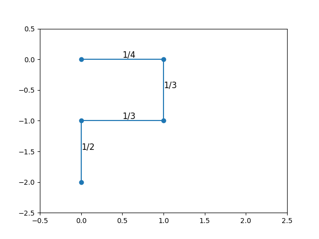
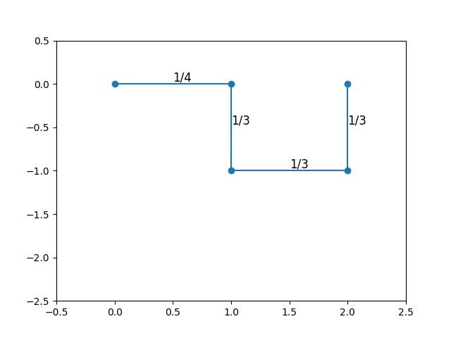
The diagrams above show two walks sampled in this way, starting at the origin, with each step probability labeled. The first three steps have the same number of choices (hence the same probability) for both walks. However, the last step has fewer options in the first walk than in the second. As a result, these two walks have different sampling probabilities, and we’re not really sampling from the uniform distribution at all.
The blocker
A significant problem in trying to understand the SAW as a process that “grows” one step at a time is that the sequence of uniform distributions that define this model at varying sizes does not form a consistent family of marginal distributions of an encompassing stochastic process. To see this, you need some idea of how many SAWs there are for varying numbers of steps. Consider the 2-dimensional case, tabulated below.
| Steps | Count | Explanation |
|---|---|---|
| 1 | 4 | Start at the origin, go anywhere |
| 2 | 12 = 3 x 4 | Go anywhere except backwards |
| 3 | 36 = 3 x 12 | Go anywhere except backwards |
| 4 | \(c_4 > 72 = 2 \times 36\) | (explained below) |
The explanation for the last row that you’ll always have at least 2 positions to move to after the first 3 steps. You might (as shown in the diagram above) get stuck with only 2 choices, but no fewer.
Exercise. Try to count the exact number of 4-step SAWs (note that it isn’t essential to the argument that follows). It isn’t necessary to write any code or exhaustively list every configuration.
Answer
100Now consider the plot on the left above, which shows one of two possible 4-step extensions of a given 3-step walk. Each of these should have probability \(1/c_4\), making the marginal probability of the 3-step walk \(2/c_4 < 1/36\), which is inconsistent with the uniform distribution over 3-step walks.
Exercise. Where does this argument fail in the case of simple random walk?
The solution
The most successful algorithm for sampling SAW, known as the pivot algorithm and developed by Madras & Sokal, is based on the idea of performing a sequence of “self-avoidance-preserving global transformations” to an existing SAW. In other words, starting with a single SAW sample, there’s a way to produce more samples. Moreover, a single SAW sample isn’t very hard to come by: You can simply use a straight line (or, as discussed above, any path with strictly increasing coordinates).
Now you might protest that a straight line is not a representative sample of the uniform distribution, and you’d be right. The idea is that, regardless of your choice of initial walk, after sufficiently many such transformations, the result will be (approximately) uniformly distributed. This is actually an instance of a more general idea, explored next.
Markov chains and Monte Carlo
This section provides a brief review of Markov chains and MCMC. Feel free to skip it if you’re already acquainted with these subjects.
Disclaimer. A thorough introduction to this topic could easily be its own post. Instead, I’ll try to just convey the most important ideas.
Markov chains. A Markov chain is a sequence of random variables \(X_0, X_1, \ldots\) modeling events at consecutive time steps, each of which contains all the information needed to predict future events. Equivalently, given the value of one random variable in this sequence \(X_t\) (“the present”), its future \(X_{t+1}\) is conditionally independent of its past \(X_0, \ldots, X_{t-1}\). This is known as the Markov property: \(P(X_{t+1} \mid X_0, \ldots, X_t) = P(X_{t+1} \mid X_t)\).
Assumptions. It’s typical to work with time-homogeneous Markov chains, i.e ones for which the transition probabilities \(p_{xy} = P(X_{t+1} = y \mid X_t = x)\) are independent of time \(t\). We’ll also assume the set of possible states is finite, so that these probabilities form a transition matrix \(p\).
Stationary distributions. Although the transition matrix describes the Markov chain’s dynamics, its full joint distribution is unknown until we provide an initial distribution \(P(X_0)\). However, under some pretty mild conditions on the transition matrix (i.e. regardless of the initial distribution), a Markov chain’s distribution \(P(X_t)\) at time \(t\) will “stabilize”, i.e. it will converge to a stationary distribution \(\pi\). You can check that the stationary distribution (if it exists), which can be thought of as a row vector, must be a solution to the equation \(\pi = \pi p\). This equation merely expresses the fact that \(\pi\) is “stable” under the action of \(p\).
Convergence to equilibrium. Under our assumption of a finite state space, there are two conditions for convergence. The first is irreducibility, i.e. that any state can be “reached” from any other with positive probability in a finite number of steps; this is just a simple non-degeneracy requirement. The second is aperiodicity, which very loosely speaking precludes cyclic patterns of behavior. An example of a periodic chain would be one that can only reach a certain state on even time steps; convergence to equilibrium for such a chain is obviously impossible since the stationary distribution is necessarily time-independent. For us, it’s sufficient to know that any chain that is allowed to remain constant for a time step (\(p_{xx} > 0\) for all states \(x\)) is aperiodic.
Example (symmetric transitions). If the transition probabilities are symmetric (\(p_{xy} = p_{yx}\)), then the uniform distribution (\(\pi_x = 1/n\)) is stationary since \(\pi_x = 1/n = (1/n) \sum_x p_{yx} = \sum_x \pi_x p_{xy} = (\pi p)_x\).
MCMC. Markov chain Monte Carlo (MCMC) turns the idea of convergence of Markov chains to their stationary distributions on its head. Given a distribution \(\mu\) from which we’d like to sample, the idea of MCMC is to construct a Markov chain that is relatively easy to simulate and that converges to \(\mu\). Then “all” you have to do is run this simulation of the chain for long enough to get (approximate) convergence. The value of the chain at that point is a sample of \(\mu\).
Question. Can we find a Markov chain with stationary distribution given by the uniform distribution over SAWs?
The pivot algorithm
I’ll cut to the chase: The pivot algorithm uses precisely such a Markov chain.
Given an initial SAW, the pivot algorithm attempts to construct a new SAW as follows:
-
Uniformly sample a lattice site on the initial SAW; you can imagine this “pivot point” as dividing the initial SAW into two segments.
-
Uniformly sample a lattice transformation (rotation, reflection, or a combination of these).
-
“Pivot” one segment about the other using this transformation.
-
Check for intersections and reject this transformation if any are found.
|
|
It’s not hard to check that this algorithm produces an irreducible, aperiodic, symmetric Markov chain over SAWs:
-
State space: By definition, this chain preserves the self-avoiding property.
-
Irreducibility: You can form any SAW from any other SAW through a sequence of appropriate pivot moves (if you’re not convinced, see Madras & Sokal, 3.5).
-
Aperiodicity: Pivot move rejection means the chain can remain constant, which rules out cycles.
-
Symmetry: Any successful pivot can be reversed by choosing the same pivot point and the inverse transform; moreover, this inverse pivot move has the same probability of occurring as the pivot move it’s inverting.
Therefore, as long as this chain is initialized with a SAW (e.g. a straight line) in the long run its distribution will approach the uniform distribution over SAWs.
Implementation
The following goes through the key aspects of the implementation in C++. For the full code (which may differ in some ways from what’s found below), refer to https://github.com/bencwallace/pivot. This repository also implements a faster version of this algorithm, to be discussed in the next post. For the version discussed below, focus on https://github.com/bencwallace/pivot/blob/master/src/walks/walk.cpp.
Lattice transforms
We need a way to characterize, represent, and sample lattice transforms (rotations, reflections, and compositions thereof). It turns out most of the work is in the characterization.
Characterization. Rigid transformations that fix the origin are characterized by orthogonal matrices, i.e. ones whose transposes are their inverses. Since they also need to preserve the square lattice, their entries can only be ±1. Since rows and columns of an orthogonal matrix must have norm 1, this means each row and column of our transformation matrices must contain a single non-zero entry equal to ±1.
Each such transformation matrix permutes the standard basis vectors and performs sign flips on some of them. Conversely, we can get such a matrix from a choice of permutation and sign flips.
Representation. A permutation of the basis vectors can be represented as a permutation of the list of indices \(0, \ldots, d - 1\). A set of sign flips can be represented as a sequence of d numbers, each equal to +1 or -1. For now, this is just a couple of d-dimensional arrays.
template <int Dim> class transform {
  std::array<int, Dim> perm_;  // Must hold a permutation of 0, ..., d - 1
  std::array<int, Dim> signs_;  // Must only contain values +1 or -1

  /* ... */
};
Arrays vs. vectors. I used arrays instead of vectors for performance reasons. I spent some time trying to get the pivot algorithm’s performance to be comparable using vectors (even playing around with custom allocators) but always found it to be too far off. I do still think this is an interesting problem worth exploring. For now, the main downside of using arrays is the compiled code will only be able to handle a bounded number of dimensions.
Given this representation, we can represent the action of a transformation on a set of coordinates.
template <int Dim> class point {
  std::array<int, Dim> coords_{};

  /* ... */
};

template <int Dim> point<Dim> transform<Dim>::operator*(const point<Dim> &p) const {
  std::array<int, Dim> coords;
  for (int i = 0; i < Dim; ++i) {
    coords[perm_[i]] = signs_[perm_[i]] * p[i];
  }
  return point<Dim>(coords);
};
Sampling. We can sample a permutation with a random shuffle and sampling the sign flips is a matter of flipping a coin \(d\) times. Both operations require a random generator, which we represent with a template parameter for now.
template <int Dim> class transform {

  /* ... */

public:
  template <typename Gen> static transform rand(Gen &gen) {
    static std::bernoulli_distribution flip_;

    std::array<int, Dim> perm;
    std::array<int, Dim> signs;
    for (int i = 0; i < Dim; ++i) {
      perm[i] = i;
      signs[i] = 2 * flip_(gen) - 1;
    }
    std::shuffle(perm.begin(), perm.end(), gen);
    return transform(perm, signs);
  }

}
Checking for intersections
The key to implementing the pivot algorithm is finding a way to check for intersections. The most obvious way to do this is to use a hash table.
Walk representation. For instance, we can represent a walk as consisting of both a vector of points and an “occupation map”, which “inverts” the vector of points by associating to each lattice site in the walk its index in the sequence of sites.
We’ll also set up the random generator at this point. The use of the mutable keyword will be discussed when defining the pivot attempt below.
struct point_hash {
  int num_steps_;

  template <int Dim> std::size_t operator()(const point<Dim> &p) const {
    std::size_t hash = 0;
    for (int i = 0; i < Dim; ++i) {
      hash = num_steps_ + p[i] + 2 * num_steps_ * hash;
    }
    return hash;
  }
};

template <int Dim>
class walk {
  std::vector<point<Dim>> steps_;
  std::unordered_map<point<Dim>, int, point_hash> occupied_;

  mutable std::mt19937 rng_;
  mutable std::uniform_int_distribution<int> dist_;

  /* ... */
};
Choice of hash function and hash map. You might notice in the full implementation on GitHub that I replaced the STL with Boost.Unordered for the hash map (see PR#82 and commit 5f078ca). This actually has a pretty noticeable impact on performance. However, it’s a drop-in replacement and the distinction isn’t terribly important to this exposition. The hash function above is one I found to be quite performant, but it certainly would be interesting to try to improve upon it. The performance plot below shows the effect of choosing different hash map implementations and different hash functions.
Pivot attempt. A pivot attempt proceeds by transforming each point past the pivot point and checking if the result is both present in the occupation map and has index less than that of the pivot point. This works because the only possible intersections are between transformed points (which come after the pivot point) and fixed points (which come before it). A minor optimization that can be used here is to skip the pivot attempt when the sampled transform is the identity transform.
template <int Dim>
point<Dim> walk<Dim>::pivot_point(int step, int i, const transform<Dim> &trans) const {
  auto p = steps_[step];
  return p + trans * (steps_[i] - p);
}

template <int Dim>
std::optional<std::vector<point<Dim>>> walk<Dim>::try_pivot(int step, const transform<Dim> &trans) const {
  if (trans.is_identity()) {
    return {};
  }

  std::vector<point<Dim>> new_points(steps_.size() - step - 1);
  for (int i = step + 1; i < steps_.size(); ++i) {
    auto q = pivot_point(step, i, trans);
    auto it = occupied_.find(q);
    if (it != occupied_.end() && it->second <= step) {
      // intersection found
      return {};
    }
    new_points[i - step - 1] = q;
  }
  return new_points;
}
Note that I’ve omitted the definitions of some simple functions, such as transform::is_identity and the addition and subtraction operators between points.
At this point, you can see how the mutable keyword was used to ensure const-correctness of the try_pivot method. A mere pivot attempt does not modify the walk’s state; but it does modify the internal state of the random generator (otherwise, the next attempt would be identical).
Comparison with Madras & Sokal. This implementation is actually slightly different from that outlined in Madras & Sokal. Instead of using a hash set as a “scratch space”, as they do, here I’m using a “scratch vector”. Moreover, their implementation iterates over transformed steps starting from the pivot point and moving “outwards” in an alternating pattern, the idea being that intersections are more likely to occur near the pivot point. However, I tested this out and found it to be slower than the implementation above.
Successful pivot. If a pivot attempt is successful (no intersections are found), the resulting list of transformed points is copied into the walk vector and the occupation map is updated accordingly.
template <int Dim>
void walk<Dim>::do_pivot(int step, std::vector<point<Dim>> &new_points) {
  for (auto it = steps_.begin() + step + 1; it != steps_.end(); ++it) {
    occupied_.erase(*it);
  }
  for (int i = step + 1; i < steps_.size(); ++i) {
    steps_[i] = new_points[i - step - 1];
    occupied_[steps_[i]] = i;
  }
}
Putting it all together
The rand_pivot method combines the elements defined above.
template <int Dim> bool walk<Dim>::rand_pivot() {
  auto step = dist_(rng_);
  auto r = transform<Dim>::rand(rng_);
  auto new_points = try_pivot(step, r);
  if (!new_points) {
    return false;
  }
  do_pivot(step, new_points.value());
  return true;
}
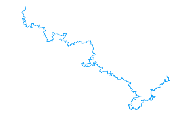
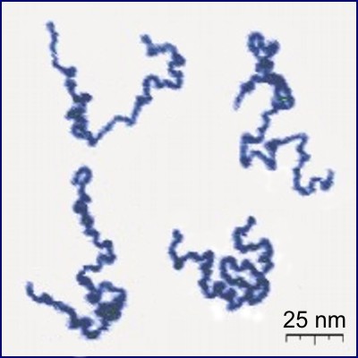
From here, all you need is a simple loop that calls rand_pivot repeatedly. When the loop ends, you can serialize the walk to a CSV file and use a python script with matplotlib to visualize it. The result, for a walk of size 105, is shown below alongside a photograph of real linear polymers taken using atomic force microscopy (AFM).
|
|
An interactive version of the plot to the left is available. I’ve also made an interactive 3D plot. Both of these were produced with plotly.
The polymer photo was found on Wikipedia, which cites the following paper:
Roiter & Minko. AFM Single Molecule Experiments at the Solid−Liquid Interface
Additional photos of polymers can be found online, for example see:
Pop, Todor-Boer, & Botiz. Visualization of Single Polymer Chains with Atomic Force Microscopy
Performance
The approximate time (in microseconds) per pivot attempt for a range of walk lengths is shown below.
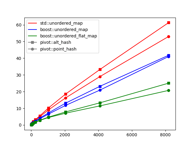
For an idea of how this plot was created, refer to the benchmark script. This script was run using different hash maps as well as different hash functions. The hash function pivot::point_hash was defined earlier. The alternative pivot::alt_hash, which uses a more standard approach to hashing sequences, is given below.
template <int Dim>
std::size_t alt_hash::operator()(const point<Dim> &p) const {
  std::size_t hash = 0;
  for (int i = 0; i < Dim; ++i) {
    hash ^= std::hash<int>{}(p[i]) + 0x9e3779b9 + (hash << 6) + (hash >> 2);
  }
  return hash;
}
An interesting problem is to explain the performance difference between these hash functions.
The bottleneck
Mathematicians and physicists who study SAW and related models are interested in their statistical properties at large scales. An example (briefly mentioned earlier) is the mean squared distance between a (uniformly random) SAW’s endpoint and the origin (its typical “size”) and how this scales with the number of steps. How can we estimate this using the pivot algorithm? Well, the plan would look something like this:
- For walk length \(n\) in some range (the bigger the better):
-
Warm up: Run very many steps of the chain (with size n) until your distribution is approximately uniform.
- For some desired sample size:
-
Record the current sample’s endpoint.
-
Run the chain for many steps so that the next sample is relatively uncorrelated from the previous one.
-
- Record the average of the squared norms of the points sampled in the previous step.
-
- Fit a curve to the data you’ve obtained.
Now every step of the Markov chain (which is run in both inner loops above) itself involves a loop over lattice sites of the walk under consideration. This loop may terminate early if the pivot attempt fails, but such attempts don’t contribute to the progress of the chain (they are wasted computation). On the other hand, successful pivot attempts involve a loop that scales linearly with the walk length.
Not all these loops necessarily scale with the size of the walk itself; but it’s not hard to believe that the warm up stage takes at least a linear number of successful iterations in \(n\), since we want a “kink” at pretty much every lattice site along the walk (see Madras & Sokal, 3.2 for a more precise argument). If you believe this, then the whole warm-up loop is of order at least \(n^2\). If we’re repeating this for \(n\) up to some \(N\), we have to do an amount of work of order at least \(N^3\).
For a more concrete sense of how long this can take, below is a chart showing the time elapsed on my laptop for varying values of the number of steps in the walk and number of iterations of the chain.
| Number of steps | Number of iterations | Elapsed time (seconds) |
|---|---|---|
| 104 | 104 | 0.66 |
| 104 | 105 | 4.79 |
| 105 | 104 | 5.00 |
| 105 | 105 | 40.22 |
| 106 | 104 | 66.51 |
The obvious bottleneck is checking for intersections. Therefore, the remaining posts will discuss how to optimize the intersection test.